Student guide: Statistics
The Statistics tab puts numbers on what the stereonet shows. It has three panels:
- Orientation statistics: the readings selected in the Filters, as one population.
- Orientation sets: the same readings split into groups (for example joint sets).
- By structure type and domain: every structure type and domain at once, each as its own population.
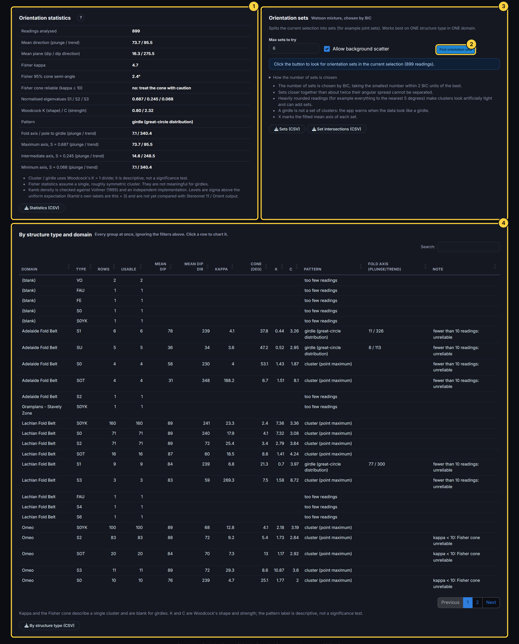
The first two panels use exactly the readings the Charts tab shows, including any rotation, unfolding, sampling-bias weights, exclusions or subset from Change the data. Settings on the Charts tab that affect statistics, such as the Confidence level and the contour method, apply here too.
The orientation matrix: where most of the numbers come from
Each reading is a unit vector: a line, or a plane’s pole. The app adds up, for every reading, the vector multiplied by itself (the outer product). The result is the 3 × 3 orientation matrix T. Its three eigenvectors are the principal axes of the data, and its three eigenvalues, divided by the number of readings, are S1, S2 and S3 (largest first), which add up to 1.
You do not need the algebra to use them. Think of the readings as a cloud of points on a sphere:
- S1 large, S2 and S3 small: the points bunch around one direction (a cluster).
- S1 and S2 similar and large, S3 small: the points spread around a great circle (a girdle).
- All three near 1/3: the points are scattered everywhere (no preferred orientation).
Because a reading and its opposite give the same product, the matrix does not care which way a pole points. That is right for orientation data.
Orientation statistics, line by line
| Statistic | What it is | How to read it |
|---|---|---|
| Readings analysed | How many readings. With sampling-bias weights, also the effective n. | Fewer than 10 and the statistics are unreliable. |
| Mean direction (plunge / trend) | The principal axis S1: the line around which the readings bunch. For planes, the mean pole. | Meaningful only for a cluster. |
| Mean plane (dip / dip direction) | For planes: the plane whose pole is the mean pole. | The “average” bedding or joint. |
| Fisher kappa | How tightly the readings bunch: (N − 1) / (N − R), where R is the length of the sum of the vectors (all turned into the mean’s hemisphere first). | Higher is tighter. Below 10 the readings are spread and the cone is unreliable. |
| Fisher 95 % cone semi-angle | The radius of the cone of confidence around the mean, at the Confidence level chosen on the Charts tab (95 % by default). | The true mean direction lies inside this cone with that confidence. It shrinks with more readings and with tighter clustering. |
| Fisher cone reliable (kappa ≥ 10) | Whether the cone can be trusted. | “no: treat the cone with caution” when the readings are too spread. |
| Normalised eigenvalues S1 / S2 / S3 | The shape of the cloud of points, as above. | See the next two rows. |
| Woodcock K (shape) | ln(S1/S2) / ln(S2/S3). | K above 1: cluster-like. K below 1: girdle-like. |
| Woodcock C (strength) | ln(S1/S3). | How strong the fabric is. C below 1 means there is no clear preferred orientation. |
| Pattern | The app’s label from K and C: cluster (point maximum), girdle (great-circle distribution) or weak or no preferred pattern. | A description, not a significance test. |
| Fold axis / pole to girdle (plunge / trend) | The eigenvector of S3: the pole to the best-fit great circle. For folded bedding, this is the fold axis. | Meaningful only for a girdle. |
| Maximum / Intermediate / Minimum axis | The three eigenvectors with their S values. | The full principal-axis description. |
| Bingham 95 % ellipse semi-axes | Only when the Bingham ellipse is on (Charts tab). The two half-widths of the confidence ellipse. | Two different values mean the cluster is elongated, which a circular Fisher cone cannot show. |
| Kamb counting circle radius and expected count / σ | Only when Kamb contours are on. The size of the counting circle for your number of readings, and what a uniform scatter would give. | Explains the σ levels on the chart. |
| Schmidt or Fisher density rows | Only when those contour methods are on. | The maximum density in that method’s units. |
Statistics (CSV) downloads the table.
Which numbers to use
The two patterns need different statistics. This is the most important idea on the tab.
| Pattern | Use | Do not use |
|---|---|---|
| Cluster (K > 1) | Mean direction or mean plane, Fisher kappa, cone of confidence. | The fold axis: it is the least-defined direction of a cluster. |
| Girdle (K < 1) | Fold axis (pole to girdle), K and C. | The mean and the Fisher cone: the mean falls between the limbs, where there may be no readings. |
| Weak (C < 1) | Report that there is no preferred orientation, and check for mixed types or domains. | Any single direction. |
As the notes under the table say: “Fisher statistics assume a single, roughly symmetric cluster. They are not meaningful for girdles.”
A worked example
Load Synthetic: joint set (cluster). The table shows (your numbers will be close to these):
- Pattern: cluster. K is well above 1.
- A mean plane, and a kappa well above 10, so the cone is reliable.
- A cone semi-angle of a few degrees: the mean joint orientation is known to within that.
Now load Synthetic: folded beds (girdle):
- Pattern: girdle. K is below 1.
- The fold axis is the direction to report.
- Kappa is low and the cone is large or unreliable, which is what you expect: the Fisher numbers do not describe a girdle.
Orientation sets
Many rocks have several joint sets, each a cluster of its own. Find orientation sets separates them.
Controls
| Control | Meaning |
|---|---|
| Max sets to try | The largest number of sets considered (1 to 8, default 6). |
| Allow background scatter | Adds a “scatter” group for readings that belong to no set. Usually leave it on: real data have random fractures. |
| Find orientation sets | Runs the search. Large selections take up to a minute. |
How the number of sets is chosen
The app fits a mixture of Watson distributions (one bell-shaped cluster per set, plus the optional uniform scatter) for 0, 1, 2 … sets. More sets always fit better, so each fit is scored with the BIC (Bayesian information criterion), which rewards a good fit but penalises extra parameters. The app takes the smallest number of sets whose BIC is within 2 of the best. The fold How the number of sets is chosen shows the score for every number of sets.
Why BIC: it stops the app inventing sets. Two sets will be separated only if the data really support two.
The results
- A message: how many sets were found, and what percentage of readings is background scatter.
- Show on the chart: All sets, or one set alone (the others grey). Clicking a row in the table does the same; clicking it again shows all the sets.
- Colour the Charts tab by set opens the Charts tab with every reading coloured by its set, so you can use the full menu (contours, downloads).
- Analyse only this set makes the chosen set the subset for every tab: its statistics, charts and report. Back to all the sets brings the sets back as you left them.
- The chart, with each set’s mean axis marked X.
- The table: each set’s readings and percentage, mean orientation, Spread (how wide the set is, in degrees) and its cone of confidence.
- For planes, Intersections of the set mean planes: where each pair of sets meets, as a plunge and trend, and the angle between them. The intersection lines of joint sets control wedge failures and the shape of blocks.
The set column is added to the Data tab and its CSV download, and to the Leapfrog table.
Sets (CSV) and Set intersections (CSV) download the tables.
Warnings, and why they appear
- “The data look like a girdle…” The set finder looks for clusters. Folded bedding spreads along a great circle; splitting it into “sets” produces artefacts. Use the fold axis instead.
- “The best model uses the maximum of N sets; there may be more.” Raise Max sets to try.
- Sets closer than about twice their spread cannot be separated. Two joint sets 10° apart, each 8° wide, look like one set to any method.
- Rounded readings (see Data health) can create false sets at round numbers.
By structure type and domain
This table runs the statistics for every structure type in every domain at once, so you can compare them side by side. It ignores which types and domains you ticked in the Filters (but uses the same columns, measurement type, strike convention, declination and confidence). It also ignores exclusions, subsets, rotation, unfolding and weighting, so it always describes your data as recorded.
| Column | Meaning |
|---|---|
| Domain, Type | The group. |
| Rows, Usable | Readings in the group, and how many passed the checks. |
| Mean dip / Mean dip dir | The group’s mean plane (or mean line). |
| Kappa, Cone (deg) | As above, for the group. |
| K, C, Pattern | Woodcock’s shape, strength and the pattern label. |
| Fold axis | For groups that are not clusters. |
| Note | “fewer than 10 readings: unreliable” or “kappa < 10: Fisher cone unreliable”. |
Click a row to chart that group: the app sets the Filters to it and opens the Charts tab. By structure type (CSV) downloads the table. Up to 60 groups are shown.
Why: a quick survey of a whole dataset. It shows which types are well defined, which domains differ, and where you have too few readings to say anything.
Reporting your statistics
A good report states:
- The number of readings (and the effective n, if weighted).
- The pattern, with K and C.
- For a cluster: the mean plane or line, kappa, and the cone semi-angle with its confidence level.
- For a girdle: the fold axis.
- The settings: projection, contour method, confidence level, strike convention, declination, and any rotation, unfolding, weighting or exclusions.
The report on the Charts tab (Export and report) does all of this for you.
Exercises
- Effect of sample size. On the Lachlan bedding demo, note kappa and the cone. Then, on the Charts tab, select about 20 readings with the box and click Use only these. How do kappa and the cone change? Which changes more, and why?
- Find the three types. Load the drillhole demo and include all three structure types (bedding, joint, fault zone). Find the orientation sets. Do the sets match the types? Compare each set’s mean with the type means in By structure type and domain.
- A girdle is not sets. Run the set finder on the folded-beds demo. What warning appears, and why?
- Confidence level. Change the confidence level on the Charts tab from 95 % to 99 %. What happens to the cone semi-angle, and why does it grow?