Identifying Outliers when Assessing Precision in Mining & Exploration
Introduction
Two methods for the statistical derivation of control lines to identify outliers when assessing precision on control charts are discussed. The first is based on Statistical Quality Control (SQC), a methodology long established in other industries, such as manufacturing. The second, known as median absolute deviation (MAD), utilises robust statistics. Both are methodologies for identifying outliers.
You should be aware that geological variation provides the largest contribution to error. Any perceived precision issues may not be due to issues in sampling or issues at the laboratory for example. That is not to say they do not exist. They do. But it may be the product, and not the process, which is mostly impacting precision. The challenge is to be able to identify these other issues and NOT fail purely because geological variation has NOT been taken into account.
The discussion and examples that follow are based on analytical results for an alumina deposit over one month (1 April 2014 to 30 April 2014 inclusive). I have purposely kept theory to a minimum.
It is crucial that a carefully designed, implemented and followed QA framework be in place for any QC assessment to be meaningful. The former represents proactive measures, the latter are reactive measures. On that note, I would like to alert you to a specialist LinkedIn group focused towards discussingQAQC issues in Mining and Exploration. I encourage you to join and share your experiences.
Statistical Quality Control
In a recent LinkedIn article, I discussed the application of statistical quality control (SQC) to the assessment of accuracy of analytical results. I also provided some background to SQC, extracts of which I present here:
The founder of SQC, Walter A. Shewart (1924), recognised that variation in a process can be divided into two fundamental components:
- Chance causes: Cumulative effect of many small, essentially unavoidable natural variability or background noise. These will always be present.
- Assignable causes: Large variability or unacceptable level of process performance that arises from sampling/human error, wrongly calibrated instruments. These are avoidable. Identifying and minimising is essential.
If a process exhibits only chance variability, it is said to be ‘in control’. If assignable causes are present, the process maybe ‘out of control’ or heading towards an out of control state. SQC is the application of statistical techniques to measure and evaluate the quality of a product, service, or process. Control is managed through control charts. Charts have upper and lower control limits derived by statistical inspection of the sample population. The process is in control if sample measurements are between the limits.
The underlying objective of SQC is to quickly detect the occurrence of assignable causes that induce a process to shift to an ‘out of control’ state, and therefore allow investigation of the process so that corrective action may be undertaken if necessary. The control chart is a process-monitoring technique (widely used in manufacturing and other industries).
It is beyond the scope of this article to provide a detailed discussion of SQC. Interested readers are encouraged to do their own research. There are many sites dedicated to SQC.
Normal Distribution
Chance causes, by their random nature, exhibit a Normal (Gaussian) Distribution. The Normal distribution is fundamental to the creation of control lines in SQC:
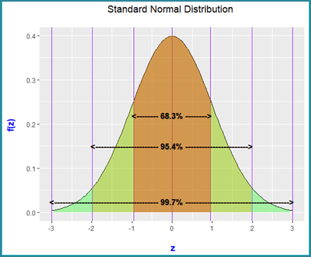
The Standard Normal distribution has the following properties:
- Bell shape (symmetric)
- Mean and median are equal and are located at the point of inflection (0)
- 95.4% of data can be expected to fall within 2 standard deviations of the mean (or no more than 4.6% can be expected to fall outside)
- 99.7% of data can be expected to fall within 3 standard deviations of the mean (or no more than 0.3% can be expected to fall outside)
There are two shape related statistics of interest:
- Skew: A measure of the asymmetry. Skewness can be positive or negative. A value of 0 indicates symmetry. Generally, where skew ranges between -0.5 and 0.5, this indicates reasonable symmetry. The larger the value, the more skewed. Skewed data implies some form of bias and will impact SQC derived control lines. More later.
- Kurtosis: A measure of the combined weight of a distribution’s tails (data at extremities) relative to the rest of the distribution. Low values indicate short tails. High values indicate long tails. A normal bell-shaped distribution is referred to as a Mesokurtic shape distribution. Platykurtic is somewhat flat and has a negative kurtosis value. A Leptokurtic distribution is more peaked, with long tails and has a positive kurtosis. You will see, as you progress through this article, that distributions are Leptokurtic (unsurprisingly). The larger the Leptokurtic value, the longer the tails. Highly Leptokurtic distributions will push SQC derived control lines away from the mean. This is an important consideration.
SQC Derived Control Lines - Relative Difference v Mean of Pairs Control Chart
Numerous methods are available for the calculation of Relative Difference (RD). The charts used in this article are based on Mean Paired Relative Difference% (MPRD%) (Pitard, 1998):
MPRD% = (a - b) / (a + b) / 2 100*
Other measures of RD exist (e.g. Bumstead, 1984, Shaw, 1997 both cited in Absalov, 2011, for example)
From an SQC perspective, MPRD% should possess a degree of normality. The chart below displays MPRD% v Mean of Pairs:
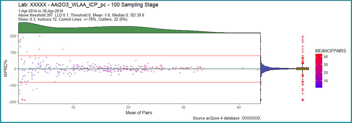
- Colour coding is based on the level of concentration (mean of pairs)
- Black is the 0-MPRD line, green horizontal line is the median and purple is mean. Because these lines are close, they mask each other
- Control lines are based on mean MPRD% +/- 2 Standard Deviations (SD). For a Normal distribution, we expect no more than 4.6% of the data to lie outside
- Outliers are flagged with a ‘cross’ symbol
- Density curves (DC) are overlaid as marginals:
o The right-hand DC relates to MPRD%
o The top DC relates to Mean of Pairs
- For reference, a Box and Whiskers is displayed. Outliers (cross symbol) on the Box and Whisker charts are based on values greater/less than:
o 75th percentile + 3 x Interquartile Range (IQR)
o 25th percentile – 3 * IQR
Comments:
- There are abundant high MPRD% values at low concentrations. This is a common (referred to as a ‘base of wine glass’ shape) phenomenon. See later.
- Mean and median are very close, indicating symmetry and possible normality. Median is 0
- 22 (6%) outliers have been identified, with the majority at low concentrations
- The density curve for MPRD% appears symmetric, with a very large concentration of values clustered close to the mean/median
- Skew indicates symmetry. The distribution is leptokurtic. Most of the data is centred close to the mean, but there are long tails. This is due to the influence of high MPRD% values at low concentrations which are influencing the SD. Control lines are being pulled away from the mean (and 0-MPRD line). Potential outliers maybe overlooked.
- The Box and Whiskers flags significantly more outliers. Some of these are more likely to be false positives.
A closer look at the MPRD% density charts for each:
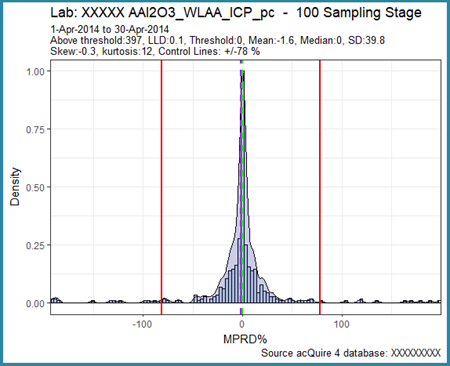
- Histogram with density curve underlaid
- Vertical lines are median (green) and mean (purple) respectively.
- Red vertical lines are 2 SD control lines
Comments:
- Very large concentration close to 0 value
- Normal distribution shape, however there are long tails (pushing the control lines away from the centre). This is also reflected in the high kurtosis (leptokurtic)
- Reasonable symmetry (important for SQC), matches the low skew.
Quantile-Quantile Chart
A Quantile-Quantile (QQ) chart is a good visual guide for normality (or otherwise). The QQ chart compares actual data with theoretical values derived from the Standard Normal curve:
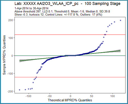
- Best-fit line shown with 95% confidence interval band
- Horizontal lines:
o median (green)
o mean (purple)
o SQC derived 2SD control lines (red)
Comments:
- For normality, the points should be located close to a straight line. This is not the case. In fact, the shape exhibited is typical of a distribution with long tails.
- Most points are located close to the best-fit line.
As the data is symmetric and the mean and median are close to 0, SQC based control lines are valid. However, the control lines are being pulled away from the mean due to the large number of outliers at low concentrations. I would be hesitant to base any decisions on these control lines.
Threshold is your friend
The high MPRD% at low concentrations (base of wine glass shape) is a common phenomenon due to the sensitivity of an instrument close to its lowest level of detection (LLD). LLD is the smallest amount of analyte that can be reliably reported. The chart below (results for the year 2013) for Laboratory Checks demonstrates the base of wine glass shape effect:
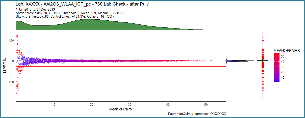
The low concentration, high MPRD% values are influencing the mean and standard deviation and therefore the control lines. Notice the hump at low concentrations for the marginal DC for Mean of Pairs at the top of the chart. We can remove the pairs causing the wine glass base by applying a threshold. Here, LLD is 0.1. Let’s apply a threshold of 1, (10 * LLD):
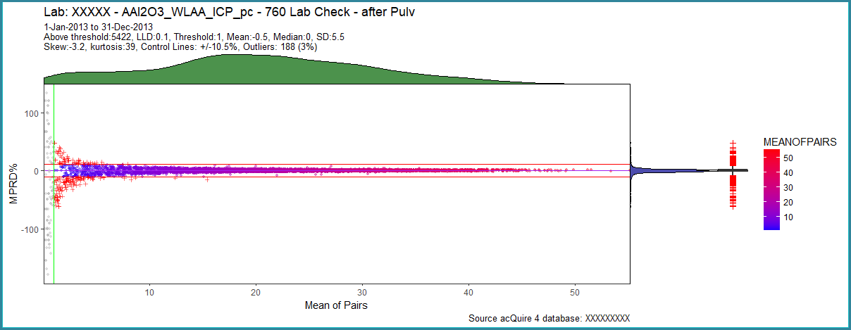
Comments:
- Extreme outliers (the wine glass base) have been removed (grey points)
- The distribution remains leptokurtic, reduced in magnitude
- Mean is close to the median and the 0-MPRD line. Median is 0
- Ignoring below threshold data removes their influence on control lines, which are now closer to the 0-MPRD line
- Number of outliers represent 3% overall
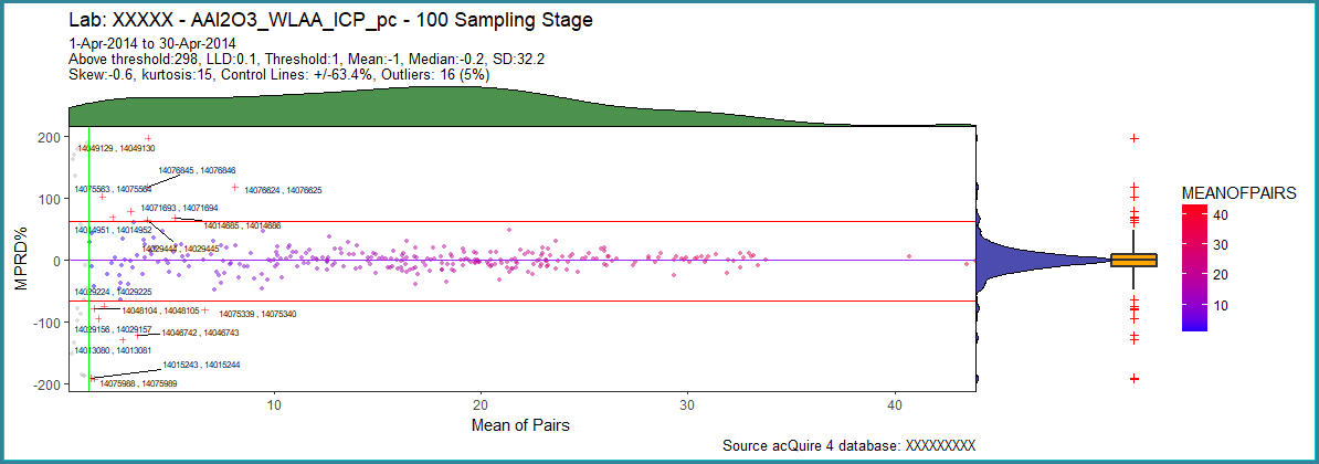
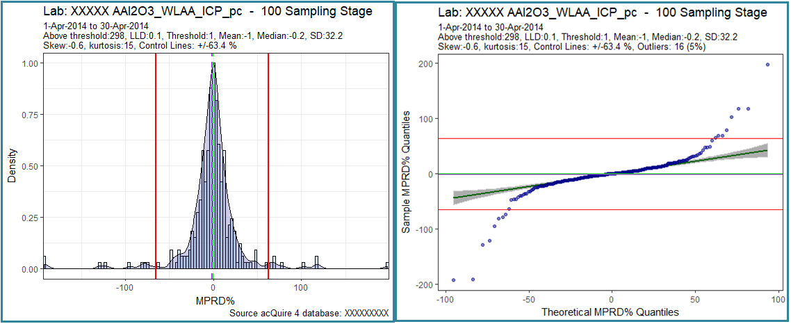
I could experiment more with threshold (for example by choosing a concentration close to the inflection point at the base of the DC Mean of Pairs hump (refer to pre-threshold chart). Returning to the original one-month data, let’s apply the same threshold to see the impact on the control lines:
Comments:
- Control lines are tighter after applying a threshold, allowing for the identification of potential outliers, although many are still at lower concentrations
- Almost symmetric with is a slight negative skew (hence mean = -1). This will pull the control lines down by the same amount.
- The mean and median remain close to the 0-MPRD line. Again, an indication of symmetry and possible normality
- On the QQ chart, the tails outside of the control lines are at low concentrations (also seen on the MPRDvMOP chart). These reflect outliers
SQC also provides a framework of rules to assess whether a process is out of control or heading towards an out of control state. One rule, utilises a property of the normal distribution, introduced earlier in this article:
- No more than 4.6% should lie outside of the mean +/- 2 standard deviations
- No more than 0.3% should lie outside of the mean +/- 3 standard deviations
Outliers in this example constitute 5%, which is only just above the 4.6% threshold for SQC at two standard deviations. Moreover, many lie at low concentrations. Not sufficient to deny acceptance in isolation.
MAD Derived Control Lines on a Relative Difference v Mean of Pairs Control Chart
MAD, like SD, is a measure of spread. Whereas SD is based on the mean (which is influenced by outliers, as we know), MAD is defined as the median of the absolute deviations from the median of the data (Leys et al, 2013). The median is a robust statistic, resistant to outliers. Beginning with the residuals (deviations) from the data’s median, MAD is the median of the residual’s absolute values:
MAD = median(|Yi – median(Yi)|)
Where Y represents values from i to n.
Calculate:
- median of all values
- absolute residuals using the value from step 1.
- median of absolute residuals from step 2.
There is an additional step. The final value is multiplied by a constant linked to the assumption of normality of the data. The constant is 1.4826 (75th percentile of the standard normal distribution). This now places the MAD SD on an equivalent scale as a Normal distribution SD. Control lines, however are created using the median:
Control Lines = Median(MPRD%) +/- 2 or 3 SD’s
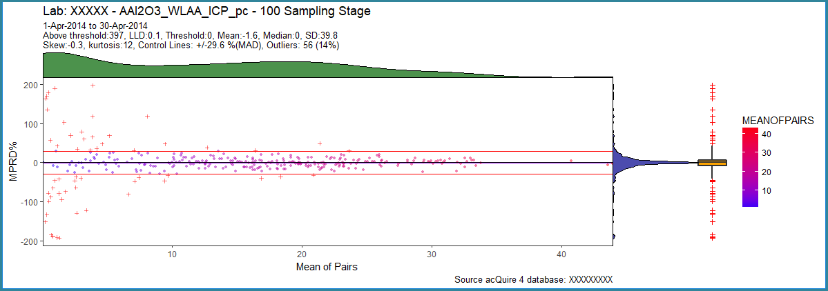
- Control lines are tighter than those created using SQC. This is because of the robust nature of MAD (no pull from outliers). In this example, I have used 3 SDs.
- For MAD control lines, even with no threshold, the high MPRD% values at low concentrations (outliers) have not impacted these control lines. There has been no need to apply a threshold.
Conclusion
SQC offers an established statistically based methodology for identifying outliers in the assessment of precision in mining and exploration, particularly with the challenges presented by geological variation (and other factors). SQC assumes a normal distribution and uses the mean and standard deviation for the establishment of control lines. Judicious use of a threshold at low concentrations may eliminate false positive outliers and, at the same time, reduce their effect on the control lines.
MAD also relies on normality of the RD statistic. Unlike SQC, control lines established using this method are resistant to the effects of outliers. As it builds control lines from the median, these are more likely to be centred around the 0-MPRD line. In general, the scaled SD is smaller than the SQC equivalent. A threshold may not be required.
If normality of the RD statistic cannot be established, then either method should be used with caution. It is important that the control lines are centred around the 0-MPRD line. If there is bias, in the case of MPRD%, this will be discernible from the chart and statistics. Control lines will be fluid over time. They should be. This reflects the inherent geological variation in the product.
Chart Source
All charts developed using the R programming language and ‘Shiny’. A cloud version is available to explore.
Resources
Acknowledgments
Ian Robertson provided valuable comments on an early draft of this article.
References
Abzalov, M. (2011). Sampling Errors and Control of Assay Data Quality in Exploration and Mining Geology. In O. Ivanov, Applications and Experiences of Quality Control. Retrieved from https://www.intechopen.com/books/applications-and-experiences-of-quality-control/sampling-errors-and-control-of-assay-data-quality-in-exploration-and-mining-geology
Bumstead, E. D. (1984). Some comments on the precision and accuracy of gold analysis in exploration. Proceedings AusIMM, 289, pp. 71-78.
Fell, P. (2017). The Application of Statistical Quality Control to Assessing Accuracy of Analytical Results. Retrieved from: https://www.linkedin.com/pulse/application-statistical-quality-control-assessing-fell-mausimm-maig/
Fell, P. (2017). The Impact of Geological Variation when Quality Controlling Precision. Retrieved from: https://www.linkedin.com/pulse/impact-geological-variation-quality-controlling-precision-paul-fell/
Leys, C., et al. (2013). Detecting outliers: Do not use standard deviation around the mean, use absolute deviation around the median. Journal of Experimental Social Psychology, 49(4), 764-766. doi:http://dx.doi.org/10.1016/j.jesp.2013.03.013
Pitard, F. F. (1998). A strategy to minimise ore grade reconciliation problems between the. Mine to Mill Confernce (pp. 77-82). Melbourne: AusIMM.
Shaw, W. J. (1997, May 16). Validation of sampling and assaying quality for bankable feasibility studies. The Resource Database Towards 2000, (pp. 69-79). Wollongong.
First published on LinkedIn, 24 April 2018. More on this topic: Duplicates; Control charts.