The Charts tab

The Charts tab in QC Analytical Results: the Charting menu on the left sets the chart type and its settings.

The Charting menu on the left sets the chart type and its settings. Its controls change with the chart you choose. Select the small ? beside a control to see what it is for, and select anywhere else to close it. The chart area shows the chart, with How this is calculated above it and its statistics below.

Chart menu: Precision

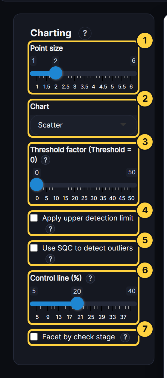
1. Point size: The size of the points on the chart.
2. Chart: The chart type. Each QC type has its own list, from scatter and RD charts to Thompson-Howarth.
3. Threshold factor: Multiplies the detection limit (LLD) to give a threshold. Pairs below it are left out of the statistics and control lines. Scatter and RD v Mean Pairs show them greyed out, and the other charts don’t draw them.
4. Apply upper detection limit: Leaves out pairs where either result is above the upper detection limit. It works only on rows that have a value in the UPPERDETECTION column.
5. Use SQC to detect outliers: Finds outliers by statistical control instead of the manual control lines. An outlier is beyond the 3 SD action limit, and the 2 SD warning band is shown too.
6. Control line (%): The relative difference, in %, at which the manual control lines are drawn.
7. Facet by check stage: Draws one panel per check stage, two across. RD v Sequence puts them one below the other.

Chart menu: Accuracy

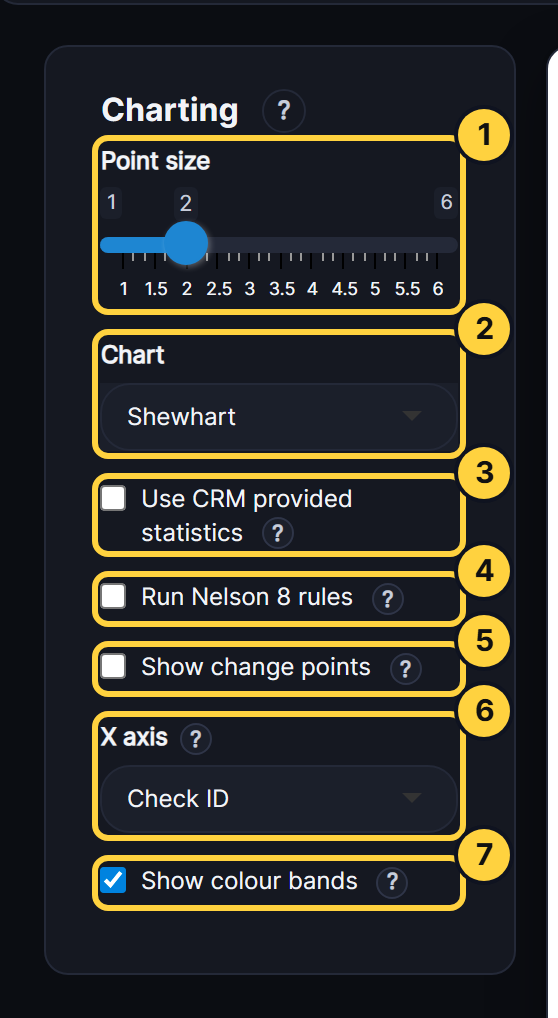
1. Point size: The size of the points on the chart.
2. Chart: The chart type: Shewhart, Cusum, Exponentially Weighted Moving Average, All Time Series, Box and whiskers or Z-Score.
3. Use CRM provided statistics: Builds the control lines from the CRM’s certified value and standard deviation, not from the results. Z-Score always centres on the certified value. For Z-Score this box changes only the standard deviation.
4. Run Nelson 8 rules: Flags runs and trends in the CRM’s results, such as nine in a row on one side of the centre line. A table lists the rules that were broken.
5. Show change points: For Shewhart and CUSUM, finds where the results shifted, by change-point analysis. A dashed purple line marks each change at 95% confidence or more. The list under the chart gives every change, and any possible one at 90 to 95%.
6. X axis: What runs along the bottom: Lab Job No, Despatch No, Check ID or Date.
7. Show colour bands: Shades the chart green within the 2 SD warning limits, amber between the warning and 3 SD action limits, and red beyond them.

Other controls

• Essential charts only: Shortens the Chart list to the core charts. For Precision these are Scatter, RD v Mean Pairs and RD v Sequence. For Accuracy they are Shewhart and Box and whiskers.
• Group by CRM: For Z-Score, puts each CRM’s results together along the X axis, one colour per CRM, with a dotted line between CRMs. Untick it to show every CRM in one sequence, with each point coloured by its band. On a Date axis the results stay in date order, so this only colours them by CRM. The ring beside the chart counts the results that passed (within ±2), had a warning (±2 to ±3) or failed (beyond ±3).
• RD to use: The relative difference formula. Here a is Sample 1 and b is Sample 2 of the pair. The choices are ARD% |a−b|/a, HARD% |a−b|/(a+b), CV% |a−b|/√2 over the mean of the pair, MPRD% (a−b) over the mean of the pair, and Hyslop’s RD, all × 100. ARD% and HARD% are always positive. MPRD% and Hyslop’s keep the sign, so a bias shows.
• Control line method: How the RD charts draw their control lines. SQC uses the mean ± standard deviations. MAD uses the median ± a robust standard deviation, which a few wild pairs don’t pull out.
• Rolling window (despatches): For RD Rolling Median, the number of despatches each point’s median covers. A longer window is smoother but slower to show a change.
• Charts to display: For RD v Density/Histogram, shows the histogram alone, or with its density curve, mean, median and control lines.
• Number of bins: For RD v Density/Histogram, the number of histogram bars. Ticked, it uses Sturges’ rule. Unticked, you set the number.
• Exclude outliers: For Density/Histogram, Quantile-Quantile and Thompson Howarth, leaves out the pairs beyond the action limits. The limits and statistics are then worked out again without them.
• What to chart: For Thompson Howarth, shows Precision v Concentration, the Thompson Howarth plot, or both.
• Additional options: Options for Thompson Howarth: log axes, forcing the line through a small intercept, robust regression (recommended), hiding the pairs, and using the median of the means instead of the mean.
• Partition window: For Thompson Howarth, the number of pairs in each group along the concentration. Thompson and Howarth suggest 11. A stage with many pairs can take a larger window.
• Weighting factor (Lambda): For EWMA, the weight the newest result gets. 0.2 is common. A smaller value is smoother and better at finding small, steady shifts.
• Number of Sigmas (L): For EWMA, the width of the control lines in standard deviations. The default is 2.5, and 3 is also common.
• Decision Interval (H): For CUSUM, how far the running sum can go, in standard deviations, before the process is out of control. The default is 3, and 4 or 5 is also common.
• Shift Detection (k): For CUSUM, the allowance in standard deviations. 0.5 suits finding a shift of 1 standard deviation.
• Chart (Contamination): The blanks chart shows each blank’s result against its detection limit.
• Warning factor (x LLD): For Contamination, the app flags a blank above this many times its detection limit.

Chart area

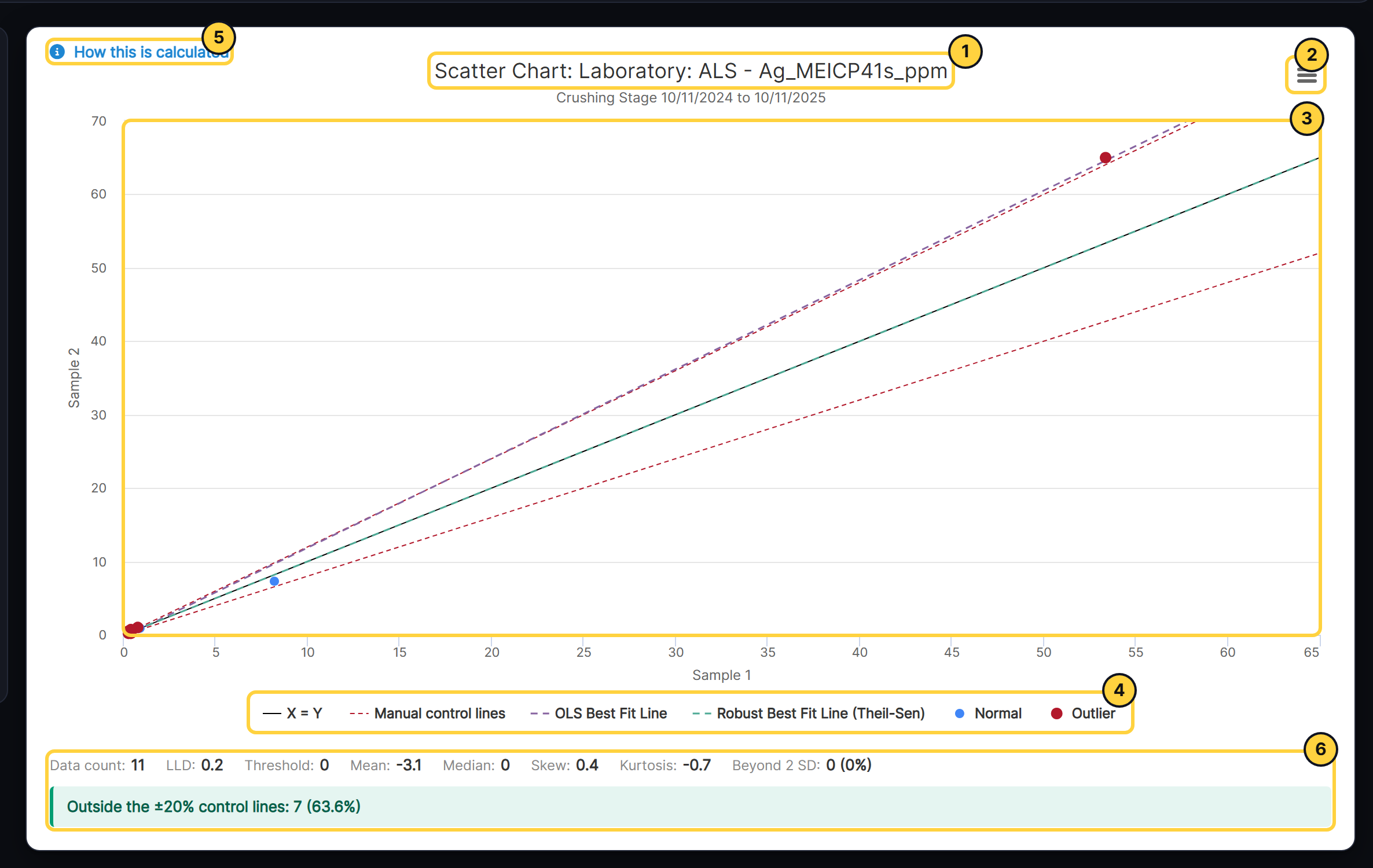
1. Title: Names the chart, laboratory and analyte, with the check stage or CRM and the dates underneath.
2. Chart menu: Opens the chart full screen, prints it, or downloads it as an image or as the data behind it.
3. The chart: Point at a result to see its details.
4. Legend: Select an item to hide or show it.
5. How this is calculated: Explains the method behind the chart, using this chart’s own numbers.
6. Statistics: Lists the chart’s statistics, with notes on what they mean, such as how many outliers to expect.